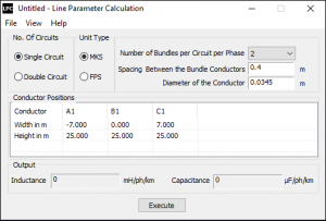
• Supports both MKS (Metric) and FPS (Imperial)
• Picks between single or double circuit line configurations.
• Customize conductor properties (bundling, spacing, diameter, position).
• Outputs include Inductance, Capacitance, GMD, GMRL, and GMRC.

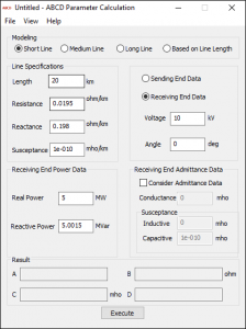
• Modeling lines as short, medium, or long based on length.
• Configurable Sending/Receiving end kV, δ, MW, MVAR and Receiving end admittance data.
• Outputs:
  • ABCD constants.
  • Line kV per km.
  • View sending-end voltage and current phasors, along with MW and MVAR values.
  • Display power factor, voltage regulation (%), and efficiency (%) for both sending and receiving ends.

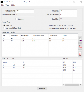
• Select cost function: normal or incremental fuel cost.
• Set total demand, number of generators, and convergence criteria for lambda-iteration method.
• Configure generator limits, cost data, and B-coefficient matrix.

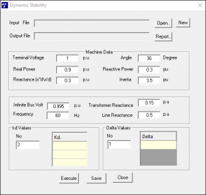
• Analyse dynamic stability with a two-machine system example.
• Customize Parameters (like machine data, infinite bus voltage, system frequency, transformer reactance and line reactance).
• Accepts Multiple input Kd and δ Values.
• Outputs dynamic coefficients and angular frequency.

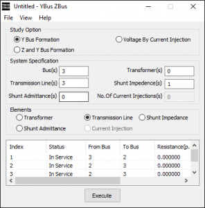
• Select study type: Y-Bus formation Y-Bus & Z-Bus formation, or Voltage by Current Injection.
• Provides fields to define full system specifications, including the number of elements and their details.
• Outputs Y-Bus, Z-Bus matrices and bus voltages (along with V ∠θ° for all buses).

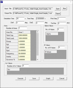
• Choose single or multi-area LFC (Load Frequency Controllers).
• Allows customization of simulation settings and area-specific details.
• Analyses how single-area frequency responds to demand changes, with or without load frequency controllers (LFCs).
• Analyses multi-area frequency and tie-line flow response when demand changes in one area.

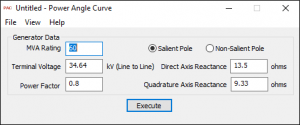
• Choose salient or non-salient pole machines.
• Configure generator rating, voltage, PF (Power Factor) and d-q axis reactance.
• Output results in machine power angles (δ) with corresponding electrical and reluctance power (MW).
• Includes an optional graph to visualize power vs. power angle for better understanding.

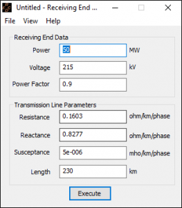
• Configure line impedance, length, receiving end power, PF (power factor), and voltage.
• Computes sending-end voltage, max real power, and power circle parameters.
• Includes power circle graph (MW vs. MVAR).

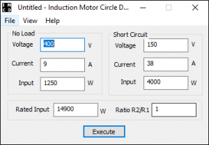
• Set voltage, current and input power values for no-load and short-circuit conditions.
• Calculates motor parameters based on rated input and stator/rotor resistance ratio.
• Shows full-load motor values, including maximum input power, output power, and torque.
• Provides a graph of the induction motor circle diagram (Real vs. Reactive power).

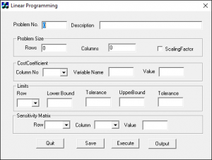
• Customize matrix size (rows and columns) and scaling factor.
• Define cost coefficient variables and their values for each column.
• Set upper and lower limits with tolerances for each row.
• Shows results including convergence status, objective function value, and linear programming solution.

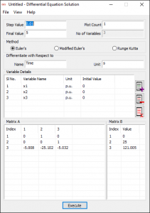
• Set the number of variables along with their units and initial values.
• Define coefficient matrices [A] and [B].
• Choose from solver methods like Euler’s, Modified Euler’s, or Runge-Kutta.
• Solves differential equations using the formula [x’] = [A] [x] + [B].
• Calculates values for each variable at every time step.
• Displays a graph showing variable values over time.

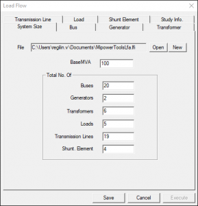
• Set basic system details including the number of elements and their specifications.
• Choose from various load flow methods like Gauss-Siedel (GS), Newton-Raphson (NR), or Fast Decoupled Load Flow (FDLF).
• Customize study parameters as needed.

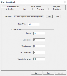
• Input basic system and fault data.
• Simulate different fault types (LLLG, LLG, LG and LL).
• Analyse faults at single/multiple buses with reactance (transient/sub-transient)

• Calculate critical clearing angle using TRS file inputs.
• Set fault clearing time, simulation times and study parameters.
• Generates a detailed report of the critical clearing angle, along with an output file for the MiPower TRS module and a graphical plot for easy analysis.

• Customize generator details such as power limits, cost coefficients, uptime/downtime, status, and start-up settings.
• Define hourly load inputs including power demand and reserve capacity.
• Select reserve type: Fixed, User Defined, or Percentage of Load.

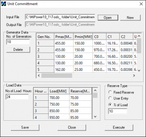
• Set the number of generators and load hours as needed.
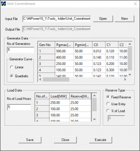
• Define generator details including power limits, cost coefficients, uptime/downtime, status, and start-up settings.
• Choose the generator cost curve type: Linear or Quadratic.
• Input hourly load data such as power demand and reserve capacity.
• Select the reserve type: Fixed, User Defined, or based on Percentage of Load.

Accordion Content

• Calculates transformer size based on its specifications and environmental conditions.
• Supports standard options: IEEE, IEC, and IS.
• Allows configuration of transformer details like HV/LV voltages, winding type, insulation (liquid/dry), cooling class, and temperature rise.
• Set installation altitude, ambient temperature, load info, and load variation factors.
• Configure HV/LV short circuit currents and Basic Insulation Level (BIL).

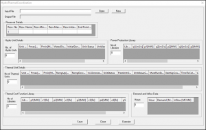
• Set reservoir details including storage limits and initial/final water levels.
• Configure hydro unit information such as unit count, power limits, output, and status.
• Use power production libraries with various volumetric flow rates and corresponding power outputs.
• Enter thermal unit details like power limits, ramp rates, initial generation, unit status, and starting parameters.
• Define thermal cost functions with multiple power outputs and corresponding costs.
• Input hourly demand and water inflow data.
• Economic Load Dispatch (ELD) for both hydro and thermal power plants.

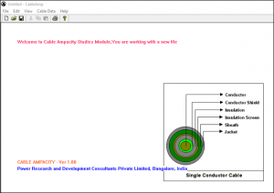
• Easy-to-use cable data editor with fully customizable input fields and settings.
• Supports both MKS (Metric) and FPS (Imperial) unit systems.
• Calculates cable ampacity based on user-defined ambient temperature (°C) limits and step size.

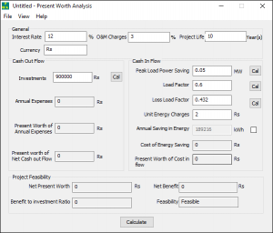
• Calculates project feasibility, net cash flow, and return on investment.
• Determines the payback period.
• Computes the project’s interest rate.
• Provides present worth results in a text format.

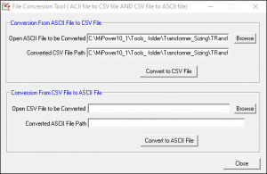
• Convert between ASCII (text) and CSV (Excel) formats for data handling.